Plotting complex variable functions
- Plotting the function’s module
- Plotting the real and imaginary part
- Domain coloring
- Conformal mapping
- Plotting as a vector field
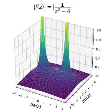
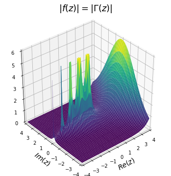
Plotting the function’s module
import numpy as np
import matplotlib.pyplot as plt
from mpl_toolkits.mplot3d import Axes3D

N = 500
lim = 4

x, y = np.meshgrid(np.linspace(-lim,lim,N),
                   np.linspace(-lim,lim,N))
z = x + 1j*y
f = abs(1/(z**2-4))
f[f>1.3] = 1.3 # Cut the function at the poles for decoration purposes.

fig = plt.figure(figsize=(6,6))
ax = fig.add_subplot(111, projection="3d", xlim=(-lim,lim), ylim=(-lim,lim), zlim=(0,1))

ax.plot_surface(x, y, f, cmap="viridis", shade=True, alpha=1)
ax.set_xlabel("$Re(z)$", size=14)
ax.set_ylabel("$Im(z)$", size=14)
ax.set_title("$|f(z)|=|\dfrac{1}{z^2-4}|$", size=18, pad=30)

plt.show()
from scipy.special import gamma

f = abs(gamma(z))
f[f>6] = 6

fig = plt.figure(figsize=(6,6))
ax = fig.add_subplot(111, projection="3d", xlim=(-lim,lim), ylim=(-lim,lim), zlim=(0,6))

ax.plot_surface(x, y, f, cmap="viridis", shade=True, alpha=1)
ax.set_xlabel("$Re(z)$", size=14)
ax.set_ylabel("$Im(z)$", size=14)
ax.set_title("$|f(z)|=|\Gamma (z)|$", size=18, pad=30)
ax.view_init(azim=-130, elev=35)

plt.show()
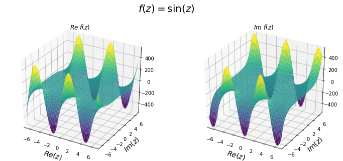
Plotting the real and imaginary part
N = 50
lim = 7

x, y = np.meshgrid(np.linspace(-lim,lim,N),
                   np.linspace(-lim,lim,N))
z = x + 1j*y
f = np.sin(z)

fig = plt.figure(figsize=(12,5))
fig.suptitle("$f(z) = \sin(z)$", fontsize=20)
ax1 = fig.add_subplot(121, projection="3d", xlim=(-lim,lim), ylim=(-lim,lim))
ax2 = fig.add_subplot(122, projection="3d", xlim=(-lim,lim), ylim=(-lim,lim))

ax1.plot_surface(x, y, f.real, cmap="viridis", shade=True, alpha=0.9, label="Re f(z)")
ax2.plot_surface(x, y, f.imag, cmap="viridis", shade=True, alpha=0.9, label="Im f(z)")

ax1.set_zlim(f.real.min(), f.real.max())
ax1.set_xlabel("$Re(z)$", fontsize=14)
ax1.set_ylabel("$Im(z)$", fontsize=14)
ax1.set_title("$Re \,\, f(z)$") # \, adds space

ax2.set_zlim(f.imag.min(), f.imag.max())
ax2.set_xlabel("$Re(z)$", fontsize=14)
ax2.set_ylabel("$Im(z)$", fontsize=14)
ax2.set_title("$Im \,\, f(z)$")

plt.show()
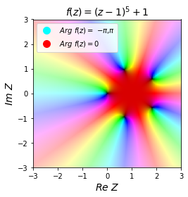
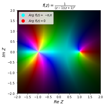
Domain coloring
from colorsys import hls_to_rgb


def colorize(fz):

    """
    The original colorize function can be found at:
    https://stackoverflow.com/questions/17044052/mathplotlib-imshow-complex-2d-array
    by the user nadapez.
    """

    r = np.log2(1. + np.abs(fz))

    h = np.angle(fz)/(2*np.pi)
    l = 1 - 0.45**(np.log(1+r))
    s = 1

    c = np.vectorize(hls_to_rgb)(h,l,s) # --> tuple
    c = np.array(c)  # -->  array of (3,n,m) shape, but need (m,n,3)
    c = np.rot90(c.transpose(2,1,0), 1) # Change shape to (m,n,3) and rotate 90 degrees

    return c


N = 500
lim = 3
x, y = np.meshgrid(np.linspace(-lim,lim,N),
                   np.linspace(-lim,lim,N))
z = x + 1j*y
f = (z-1)**5+1


from matplotlib.lines import Line2D

legend_elements = [Line2D([0], [0], marker='o', color='cyan', label='$Arg$ $f(z) =$ $-\pi$,$\pi$', markersize=10, lw=0),
                   Line2D([0], [0], marker='o', color='red', label='$Arg$ $f(z)=0$', markersize=10, lw=0)]

# Create the figure
fig, ax = plt.subplots()
ax.legend(handles=legend_elements, loc='upper left')

img = colorize(f)
ax.imshow(img, extent=[-lim,lim, -lim,lim])
ax.set_xlabel("$Re$ $Z$", fontsize=14)
ax.set_ylabel("$Im$ $Z$", fontsize=14)
ax.set_title(r"$f(z)=(z-1)^5+1$", fontsize=14)

plt.tight_layout()
plt.show()
lim = 2
x, y = np.meshgrid(np.linspace(-lim,lim,N),
                   np.linspace(-lim,lim,N))
z = x + 1j*y

f = 1/((z-1)*(z+1)**2)

fig, ax = plt.subplots(figsize=(5,5))
ax.legend(handles=legend_elements, loc='upper left')

img = colorize(f)
ax.imshow(img, extent=[-lim,lim, -lim,lim])
ax.set_xlabel("$Re$ $Z$", fontsize=14)
ax.set_ylabel("$Im$ $Z$", fontsize=14)
ax.set_title(r"$f(z)=\frac{1}{(z-1)(z+1)^2}$", fontsize=14)

plt.tight_layout()
plt.show()
#__exp(1/z)___________________________________________
lim = 1
x, y = np.meshgrid(np.linspace(-lim,lim,N),
np.linspace(-lim,lim,N))
z = x + 1j*y
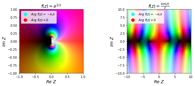
f = np.exp(1/z)
fig, (ax, ax2) = plt.subplots(1,2,figsize=(10,4))
ax.legend(handles=legend_elements, loc='upper left')
img = colorize(f)
ax.imshow(img, extent=[-lim,lim, -lim,lim])
ax.set_xlabel("$Re$ $Z$", fontsize=14)
ax.set_ylabel("$Im$ $Z$", fontsize=14)
ax.set_title(r"$f(z)=e^{1/z}$", fontsize=14)
#__sin(z)/z___________________________________________
lim = 10
x, y = np.meshgrid(np.linspace(-lim,lim,N),
np.linspace(-lim,lim,N))
z = x + 1j*y
f = np.sin(z)/z
ax2.legend(handles=legend_elements, loc='upper left')
img = colorize(f)
ax2.imshow(img, extent=[-lim,lim, -lim,lim])
ax2.set_xlabel("$Re$ $Z$", fontsize=14)
ax2.set_ylabel("$Im$ $Z$", fontsize=14)
ax2.set_title(r"$f(z)=\frac{\sin(z)}{z}$", fontsize=14)
plt.tight_layout()
plt.show()
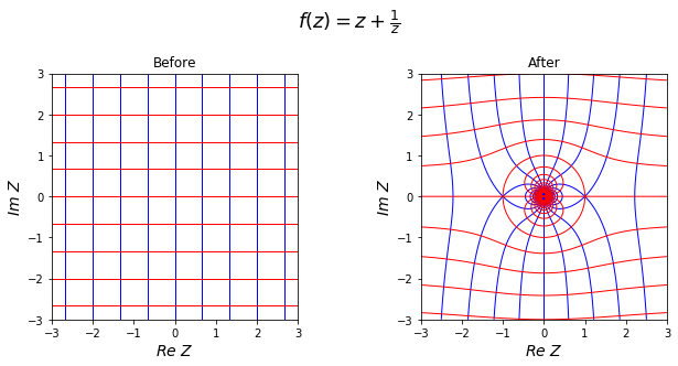
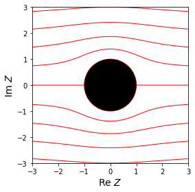
Conformal mapping
\(f(z) = \mbox{Re} f(z) + i \, \mbox{Im} f(z)\)
\[\begin{align} \mbox{Re} f(z) & = C_1 \\ \mbox{Im} f(z) & = C_2 \end{align}\]def f(z):
return z + 1/z
# The x and y coordinates
lim = 3
N = 300
Xv = np.linspace(-lim, lim, N)
Yv = np.linspace(-lim, lim, N)
X, Y = np.meshgrid(Xv, Yv)
# Values of f as a function of z=x+iy
Z = X+1j*Y
Fv = f(Z)
lv = np.linspace(-10,10,31)
# Contours of constant Re f(z) and Im f(z) as a function of x and y
fig, (ax, ax2) = plt.subplots(1,2,figsize=(10,5))
fig.suptitle(r"$f(z)=z+\frac{1}{z}$", fontsize=18)
ax.set_aspect("equal")
ax2.set_aspect("equal")
ax.contour(Xv, Yv, X, colors='blue', linestyles='solid', levels=lv, linewidths=1)
ax.contour(Xv, Yv, Y, colors='red', linestyles='solid', levels=lv, linewidths=1)
ax.set_xlabel("$Re$ $Z$", fontsize=14)
ax.set_ylabel("$Im$ $Z$", fontsize=14)
ax.set_title("Before")
ax2.contour(Xv, Yv, np.real(Fv), colors='blue', linestyles='solid', levels=lv, linewidths=1)
ax2.contour(Xv, Yv, np.imag(Fv), colors='red', linestyles='solid', levels=lv, linewidths=1)
ax2.set_xlabel("$Re$ $Z$", fontsize=14)
ax2.set_ylabel("$Im$ $Z$", fontsize=14)
ax2.set_title("After")
plt.subplots_adjust(wspace=0.5)
plt.show()
from matplotlib.patches import Circle

fig, ax = plt.subplots()
ax.set_aspect("equal")

Circ = Circle((0,0), radius=1, facecolor="black", alpha=1, zorder=10)
ax.add_patch(Circ)

ax.contour(Xv, Yv, np.imag(Fv), colors='red', linestyles='solid', levels=lv, linewidths=1)
ax.set_xlabel("Re $Z$", fontsize=14)
ax.set_ylabel("Im $Z$", fontsize=14)

plt.tight_layout()
plt.show()
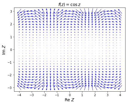
Plotting as a vector field
def f(z):
    return np.cos(z)


# The x and y coordinates
lim = 3
N = 30
Xv = np.linspace(-lim-1, lim+1, N)
Yv = np.linspace(-lim, lim, N)
X, Y = np.meshgrid(Xv, Yv)

# Values of f as a function of z=x+iy
Z = X+1j*Y
Fv = f(Z)
lv = np.linspace(-10,10,31)

# Plotting part
fig, ax = plt.subplots(figsize=(6,5))
ax.set_aspect("equal")
ax.set_xlabel("Re $Z$", fontsize=14)
ax.set_ylabel("Im $Z$", fontsize=14)
ax.set_title(r"$f(z)=\cos \, z$", fontsize=14)
ax.quiver(X, Y, np.real(Fv), np.imag(Fv), color='blue', pivot="middle", norm=True, headwidth=6, headlength=7 )


plt.tight_layout()
plt.show()
References
-
C. Fernández González (n.d.). ¿Cómo representar funciones en variable compleja? [online]. Portal.uned.es. Available at: http://portal.uned.es/pls/portal/docs/PAGE/UNED_MAIN/LAUNIVERSIDAD/
UBICACIONES/01/DOCENTE/CARLOS_FERNANDEZ_GONZALEZ/
VARIABLE%20COMPLEJA%20GEOGEBRA/REPRESENTARVC.PDF -
C. Maggi, et al. (n.d.). Aplicaciones gráficas de funciones complejas. [online] academia.edu. Available at: https://www.academia.edu/2211067/Aplicaciones_gr%C3%A1ficas_de_funciones_complejas
-
G. Viswanathan (2014). Domain coloring for visualizing complex functions. [online] Gandhi Viswanathan’s Blog. Available at: https://gandhiviswanathan.wordpress.com/2014/10/07/domain-coloring-for-visualizing-complex-functions/
-
En.wikipedia.org. (2019). Domain coloring. [online] Available at: https://en.wikipedia.org/wiki/Domain_coloring
-
Wikidot.com. (n.d.). The Casorati-Weierstrass theorem. [online] Available at: http://mathonline.wikidot.com/the-casorati-weierstrass-theorem
-
N. Hall. (2018). Conformal mapping, Joukowsky transformation. [online] grc.nasa.gov. Available at: https://www.grc.nasa.gov/www/k-12/airplane/map.html
-
S. Ganguli. (2008). Conformal Mapping and its Applications. [online] Iiserpune.ac.in. Available at: http://www.iiserpune.ac.in/~p.subramanian/conformal_mapping1.pdf