The Hong-Ou-Mandel effect
Along with quantum superposition and quantum entanglement, quantum interference is one of the most important phenomena used in quantum information processing or quantum computing. In this case, quantum interference refers to the interference of probability amplitudes. However, it is not always mentioned when discussing such topics 1.
One example of quantum interference is the Hong-Ou-Mandel effect (i.e., the HOM effect), which is of great importance in linear optical quantum computing. This type of interference occurs when two photons with identical properties enter a balanced beam splitter at the same time through different ports. Due to the indistinguishability of the photons, the probability amplitudes of the possible outcomes interfere destructively. This results in a bunching of the photons, or photon bunching. That is, the only possible outcomes are the ones where the photons travel through the same path.
The theory
Now, we will take a look at the main idea behind this effect. We will start by considering a simple quantum description of a balanced beam splitter. A balanced beam splitter is a device that reflects the 50% of the incoming light and transmits the other 50%. At the quantum level, this means that a photon will be reflected with 50% probability and transmitted with 50% probability.
For the mathematical treatment in this post, we will consider the matrix description in the second quantization formalism. That is, we will use ladder operators ($\hat{a}$, $\hat{a}^\dagger$) to show the form of the matrix describing the beam splitter as an operator. We will use Dirac notation to represent as $\vert n\rangle_a$ the presence of $n$ photons in a spatial path $a$. This way, by $\vert m\rangle_a \vert n\rangle_b$ we will mean that there are $m$ photons traveling through the path $a$ and $n$ photons traveling through the path $b$. With this, the ladder operators work as follows:
\[\begin{array}{c} \hat{a}^\dagger_a \vert n\rangle_a = \sqrt{n+1} \vert n+1\rangle_a \\[1ex] \hat{a}_a \vert n\rangle_a = \sqrt{n} \vert n-1\rangle_a \end{array},\]where the creation and anihilation operators $\hat{a}^\dagger_a$ and $\hat{a}_a$ would act on path $a$. To give some examples, we would have
\[\begin{array}{c} \hat{a}^\dagger_a \vert 0\rangle_a = \vert 1\rangle_a \;,\\[1ex] \hat{a}_a \vert 1\rangle_a = \vert 0\rangle_a \;, \\[1ex] \hat{a}^\dagger_b \vert 0\rangle_a \vert 0\rangle_b = \vert 0\rangle_a \vert 1\rangle_b \;. \end{array}\]We must also take into account that there is a relative phase between the reflected and transmitted light 2. Therefore, if the relative phase acquired by the reflected light that came through one input port of the beam splitter is $\Delta\theta_{1}$ and the one acquired by the reflected light that came through the other input port is $\Delta\theta_{2}$, they must satisfy $\Delta\theta_{1} + \Delta\theta_{2} = \pm\pi$ 3. Typically, there are two popular cases in the literature: if the beam splitter is symmetric in phase shifts, $\Delta\theta_{1} = \Delta\theta_{2} = \pm\pi/2$; if the beam splitter is not symmetric in phase shifts, $\Delta\theta_{1} = \pm\pi$ and $\Delta\theta_{2} = 0$ or $\Delta\theta_{1} = 0$ and $\Delta\theta_{2} = \pm\pi$ 4.
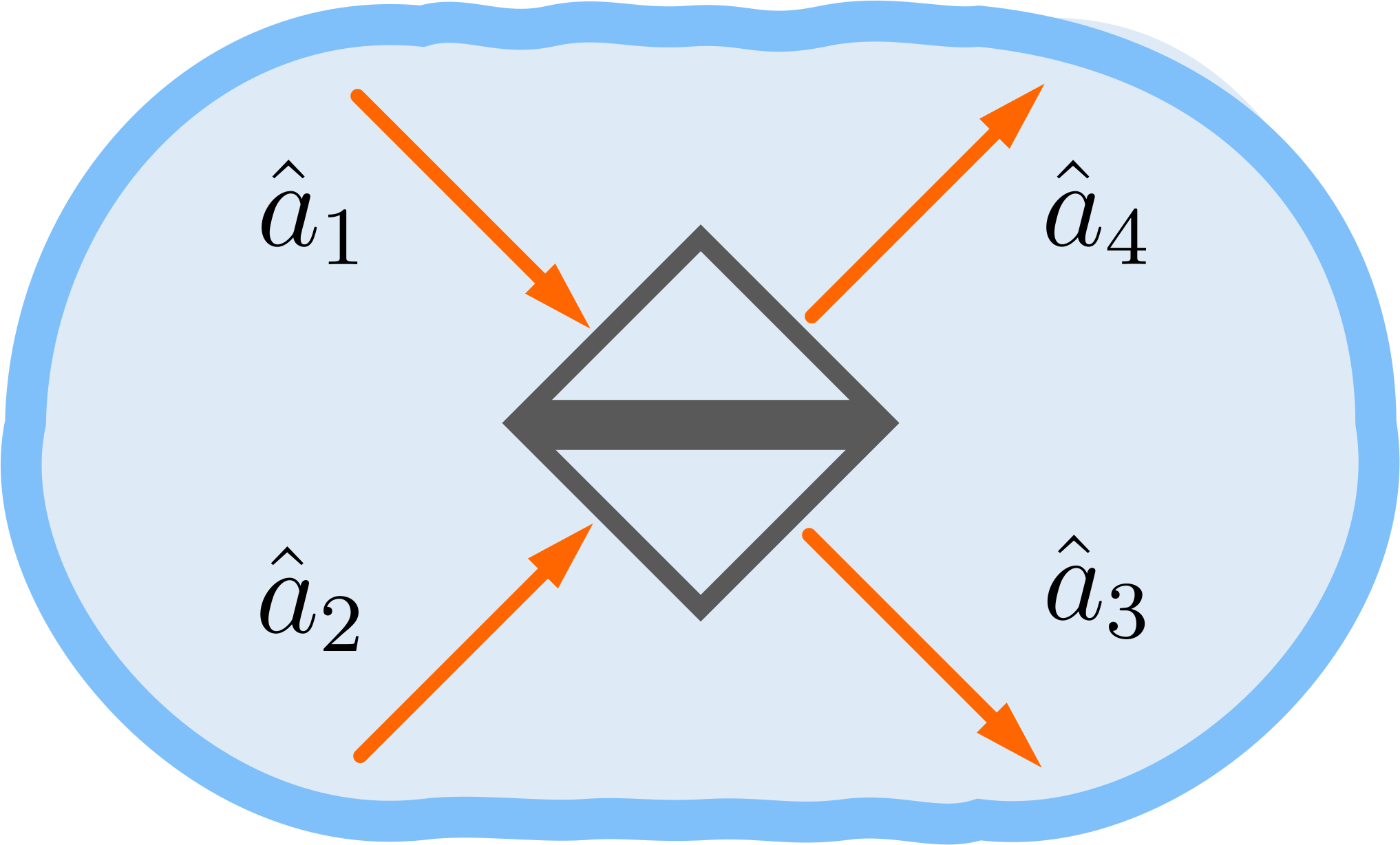
With all of this, the action of a beam splitter would be represented with ladder operators as follows:
\[\begin{array}{c} \hat{a}^\dagger_3 = t \hat{a}^\dagger_1 + re^{i\Delta\theta_1} \hat{a}^\dagger_2 \;, \\[1ex] \hat{a}^\dagger_4 = re^{i\Delta\theta_2} \hat{a}^\dagger_1 + t \hat{a}^\dagger_2 \;, \end{array}\]where $t$ and $r$ are the transmissivity and reflectivity amplitudes of the beam splitter. We can write the action of a beam splitter in matrix form as follows:
\[\begin{pmatrix} \hat{a}^\dagger_3 \\[1ex] \hat{a}^\dagger_4 \end{pmatrix} = \begin{pmatrix} t & re^{i\Delta\theta_1} \\[1ex] re^{i\Delta\theta_2} & t \end{pmatrix} \begin{pmatrix} \hat{a}^\dagger_1 \\[1ex] \hat{a}^\dagger_2 \end{pmatrix},\]with the beam splitter matrix being
\[B = \begin{pmatrix} t & re^{i\Delta\theta_1} \\[1ex] re^{i\Delta\theta_2} & t \end{pmatrix} .\]Using $r=t=1/\sqrt{2}$ for the case of a balanced beam splitter, we can write this $B$ matrix, for example, as
\[\begin{array}{ll} B = \dfrac{1}{\sqrt{2}}\begin{pmatrix} 1 & i \\ i & 1 \end{pmatrix} & \text{for } \Delta\theta_{1} = \Delta\theta_{2} = \pi/2 \,, \\[3ex] B = \dfrac{1}{\sqrt{2}}\begin{pmatrix} 1 & -1 \\ 1 & 1 \end{pmatrix} & \text{for } \Delta\theta_{1} = \pi \,\text{ and }\, \Delta\theta_{2} = 0 \,. \end{array}\]If we added the relative phases to the transmission components instead of the reflection components, we would obtain that the balanced beam splitter is equivalent to a Hadamard matrix for the $\Delta\theta_{1} = 0,\, \Delta\theta_{2} = \pi$ case:
\[B = \dfrac{1}{\sqrt{2}}\begin{pmatrix} 1 & 1 \\ 1 & -1 \end{pmatrix} .\]We will use the input-output relations of the ladder operators given by this form of the $B$ matrix for the following HOM effect calculations. The input ladder operators can be written as a function of the output operators by using
\[\begin{pmatrix} \hat{a}^\dagger_1 \\[1ex] \hat{a}^\dagger_2 \end{pmatrix} = \dfrac{1}{\sqrt{2}}\begin{pmatrix} 1 & 1 \\[1ex] 1 & -1 \end{pmatrix} \begin{pmatrix} \hat{a}^\dagger_3 \\[1ex] \hat{a}^\dagger_4 \end{pmatrix},\]where we used that our chosen $B$ matrix satisfies $B=B^{-1}$. Therefore, if we have an input state $\vert\Psi\rangle_{in} = \vert 1\rangle_1 \vert 1\rangle_2$, we can calculate the output $\vert\Psi\rangle_{out}$ by using the previous relation.
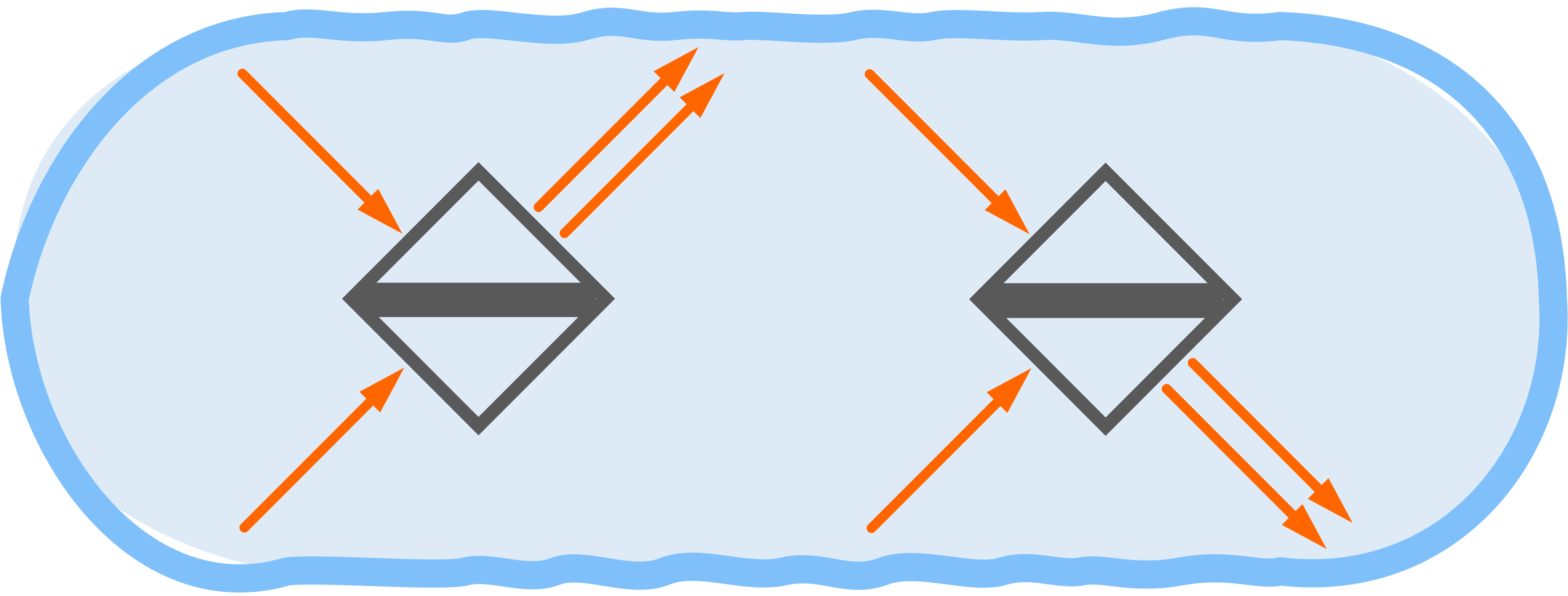
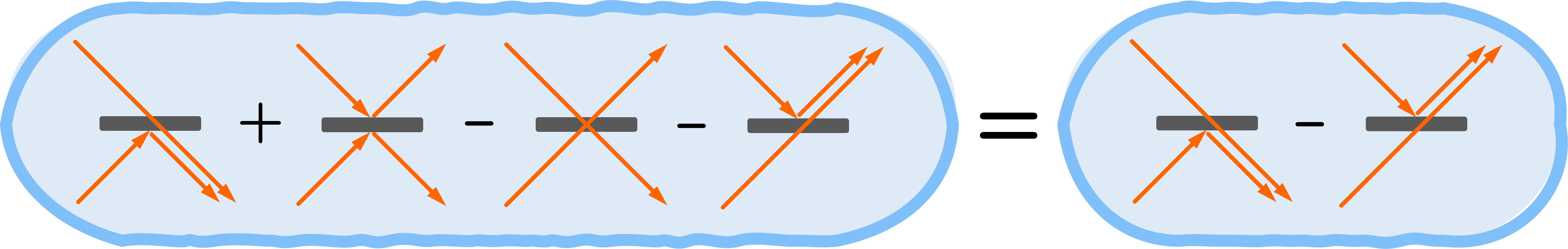
\[\begin{array}{ll} \vert\Psi\rangle_{in} \!\!\!\! & = \vert 1\rangle_1 \vert 1\rangle_2 \\[1ex] &= a^\dagger_1 a^\dagger_2 \vert 0\rangle_1 \vert 0\rangle_2 \\[2ex] \vert\Psi\rangle_{out} \!\!\!\! &= \frac{1}{2}(a^\dagger_3 + a^\dagger_4)(a^\dagger_3 - a^\dagger_4) \vert 0\rangle_3 \vert 0\rangle_4\\[1ex] &= \frac{1}{2}(a^{\dagger 2}_3 + a^\dagger_4 a^\dagger_3 - a^\dagger_3a^\dagger_4 - a^{\dagger 2}_4) \vert 0\rangle_3 \vert 0\rangle_4\\[1ex] &= \frac{1}{\sqrt{2}}(a^{\dagger 2}_3 - a^{\dagger 2}_4) \vert 0\rangle_3 \vert 0\rangle_4\\[1ex] &= \frac{1}{\sqrt{2}}(\vert 2\rangle_3 \vert 0\rangle_4 - \vert 0\rangle_3 \vert 2\rangle_4) \\[1ex] \end{array}\]These calculations can be described visually by Figure 3. We can see that the case where both photons are transmitted interferes destructively with the case where both photons are reflected. This results in a cancellation of said components, leaving behind the bunched cases where the photons exit through the same port of the beam splitter. With this, we have an output state that is entangled.
The experiments
We have seen the basic theory behind the HOM effect. Now, we will dive a bit into the original experiment by Chung Ki Hong, Zheyu Ou and Leonard Mandel.
The experimental setup is depicted in Figure 4 5. We start by pumping a laser with frequency $\omega_0$ at a KDP crystal (potassium dihydrogen phosphate crystal). This generates, with some efficiency, two photons per incoming laser photon. These two new photons have lower frequencies compared with that of the incoming photon. If one frequency is $\omega_1$ and the other is $\omega_2$, these satisfy $\omega_0=\omega_1+\omega_2$ via energy conservation. This process is known as spontaneous parametric down conversion (SPDC). In this case, we will be dealing with output photons with frequencies that satisfy $\omega_1=\omega_2=\omega_0/2$. Nevertheless, it is important to note that these photons will have some frequency bandwidth.
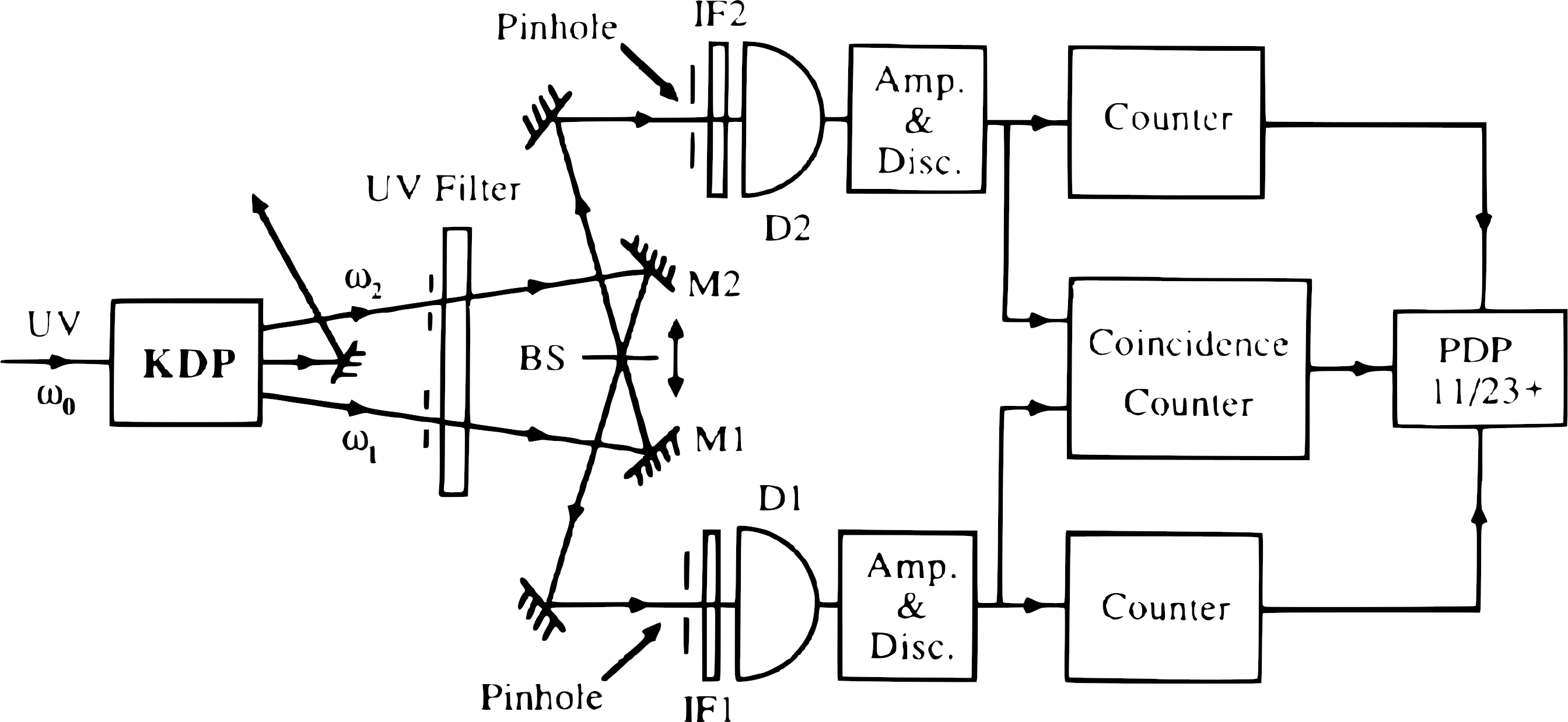
As mentioned before, with the KDP crystal we generate photon pairs. But this process is not 100% efficient, so we will also need to discard the residual (or unconverted) pump laser photons with frequency $\omega_0$. The output state after this part will be a Fock state of the form
\[\vert\psi\rangle_{KDP}=\vert 1\rangle_{L} \vert 1\rangle_{U},\]where the subindices $L$ and $U$ indicate the path taken by the photon. That is, we have one photon at the lower path, $L$, and other at the upper path, $U$, both with frequency $\omega_0/2$ in this case.
After this photon pair generation process, the photons are introduced into a beam splitter, BS, where their probability amplitudes interfere as indicated in the previous section. The resulting entangled state has the form
\[\vert\psi\rangle_{BS}=\frac{1}{\sqrt{2}}(\vert 2\rangle_L \vert 0\rangle_U - \vert 0\rangle_L \vert 2\rangle_U)\]Lastly, the photons reach the detectors D1 and D2 and a coincidence counter processes the detections. In addition, by changing the position of the beam splitter, we are able to introduce a time delay (a path difference). This delay changes the temporal distinguishability of the photons and allows to visualize the interference pattern of this experiment.
In Figure 5 the number of coincidences is shown as a function of this delay or path difference. We can see a very characteristic interference pattern, which is known as the HOM dip.
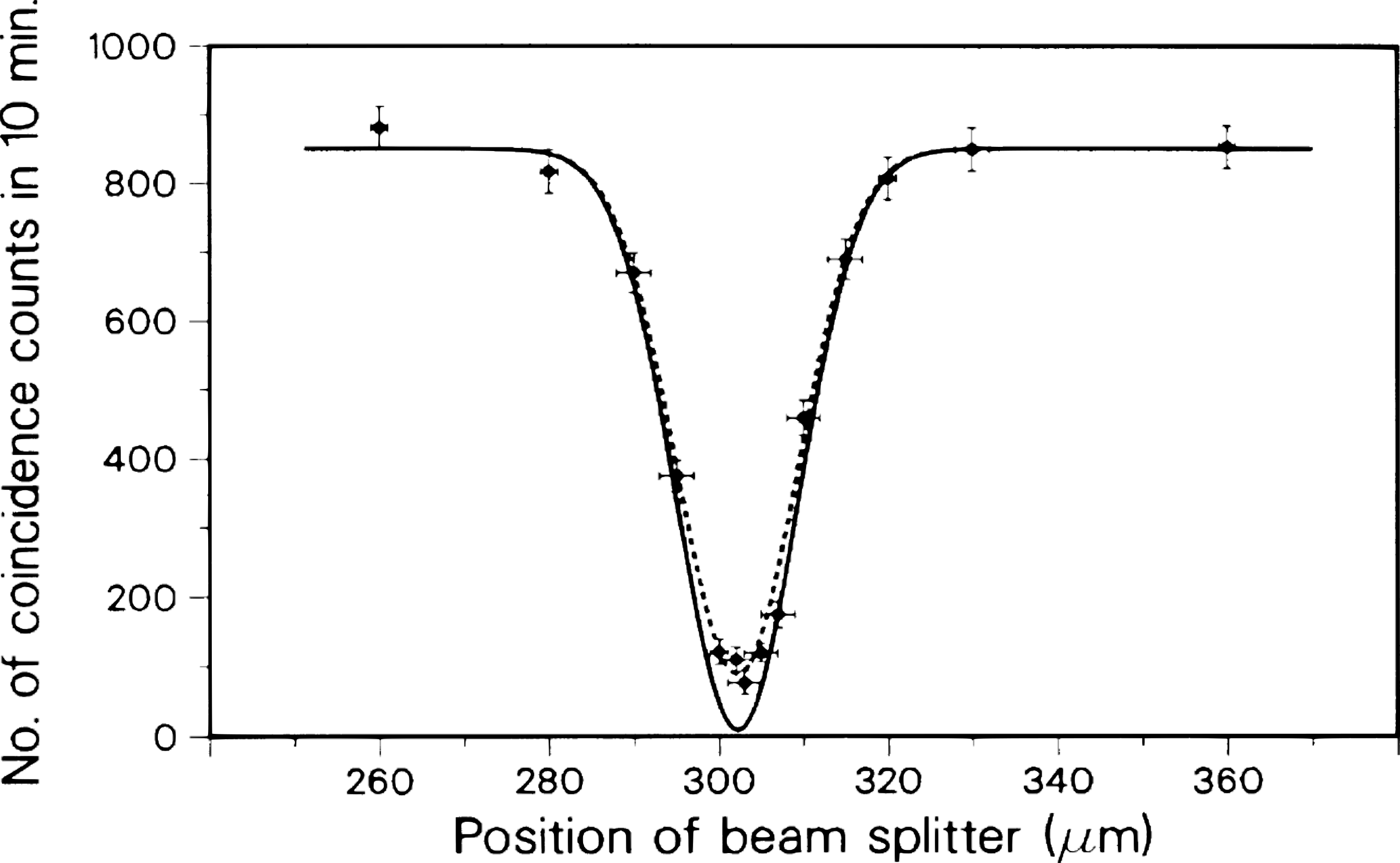
What we can see in this figure is that when we set the position of the beam splitter so that the time delay is zero (i.e., fully indistinguishable photons), the coincidence counts corresponding to the $\vert 1\rangle_{L} \vert 1\rangle_{U}$ state drop to zero. This is indicative of full interference of probability amplitudes and that the output state is $\vert\psi\rangle_{BS}$.
And the subtleties
What if the photons come from different light sources? What if the photons have different frequencies? Can we still have quantum interference?
The first question can be answered by considering that the wave function of the photons immediately before entering the beam splitter has the form $\vert\psi\rangle= \vert T_L\rangle_L \vert T_U\rangle_U$, with the single-photon wave functions being
\[\vert T_j\rangle_j = \int d\omega \,\phi_j(\omega) e^{i\omega T_j} \hat{a}^\dagger_j(\omega) \vert 0\rangle.\]Here, $T_j$ ($j=L,U$) is the arrival time of the photon $j$ at the beam splitter, $\hat{a}^\dagger_j(\omega)$ is the creation operator of a photon with frequency $\omega$ and $\phi_j(\omega)$ is the mode function giving the probability amplitude of the state component with frequency $\omega$. With the purpose of being brief, I will not go into too much detail regarding the mathematical calculations, but the answer is that we can still have HOM interference with photons from independent sources. With the wave functions above, following the mathematical derivation shown at reference 6, we can see that the visibility $\mathcal{V}$ of the HOM dip is given by:
\[\mathcal{V}(T_L-T_U-D/c)=\left|\int d\omega \phi_L^*(\omega)\phi_U(\omega)e^{i\omega (T_L-T_U-D/c)}\right|^2\leq 1,\]where $D/c$ is the delay introduced by changing the position of the beam splitter by a distance $D$. When the paths are balanced with $D/c=T_L-T_U$, it can be more clearly seen that the visibility depends on the mode overlap:
\[\mathcal{V}(0)=\left|\int d\omega \phi_L^*(\omega)\phi_U(\omega)\right|^2\leq 1.\]The equal sign is reached when the mode functions satisfy $\phi_L(\omega)=\phi_U(\omega)$ or when we have complete mode match between the two input photons.
Now, we will address the second question. With a very similar setup to the one of the previous section but where the SPDC process generates photons with different central frequencies, we can also measure interference. However, in this case, we will observe a beating pattern as shown in Figure 6.
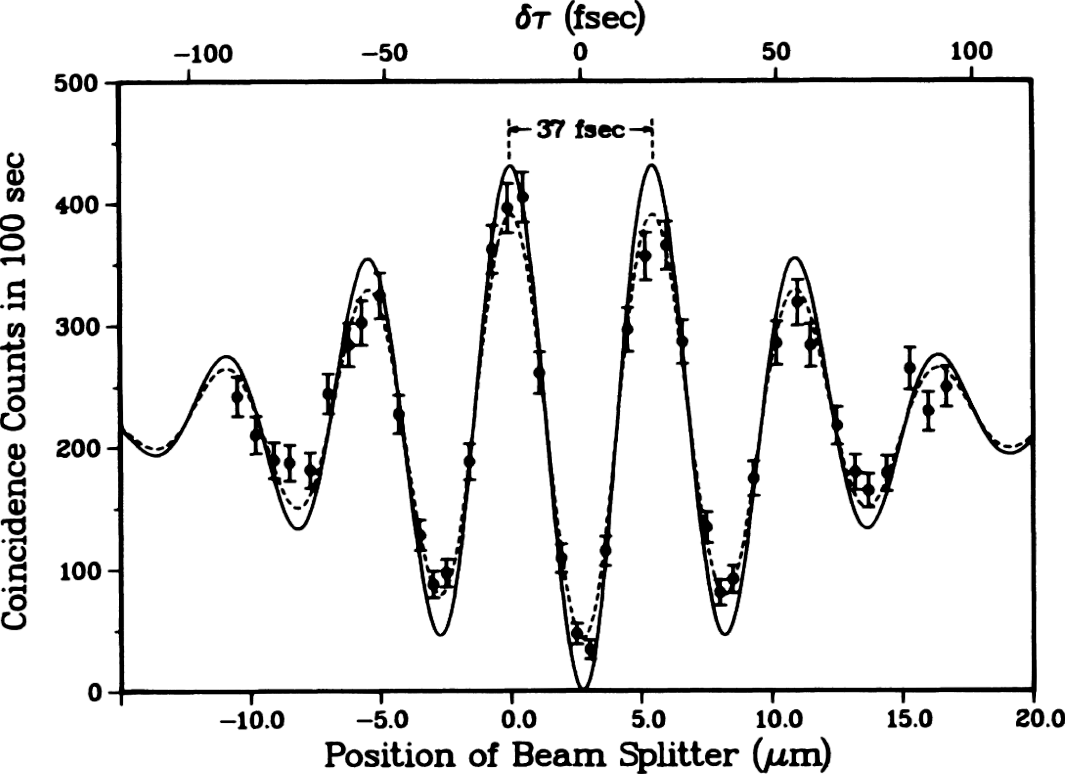
Said pattern is the result of the experiment described in reference 7. There, the photons have central frequencies $\omega_1=\omega$ and $\omega_2=\omega_0-\omega$. An additional difference between the setup of this experiment and the one described in the previous section is that the two interference filters IF1 and IF2 shown in Figure 4 are centered on different frequencies this time. These frequencies are $\omega_1$ for IF1 and $\omega_2$ for IF2. Furthermore, the passbands of the filters do not overlap. This way, it is sure that different frequency components are being measured.
References 
-
Classiq Technologies. (2022). Interference in quantum computing. Classiq. https://www.classiq.io/insights/interference-in-quantum-computing ↩
-
Hénault, F. (2015). Quantum physics and the beam splitter mystery. In The Nature of Light: What are Photons? VI (Vol. 9570, pp. 199-213). SPIE. ↩
-
Zeilinger, A. (1981). General properties of lossless beam splitters in interferometry. American Journal of Physics, 49(9), 882-883. ↩
-
G.C. (https://physics.stackexchange.com/users/143179/g-c), Phase added on reflection at a beam splitter?, URL (version: 2019-07-31): https://physics.stackexchange.com/q/494573 ↩
-
Hong, C. K., Ou, Z. Y., & Mandel, L. (1987). Measurement of subpicosecond time intervals between two photons by interference. Physical review letters, 59(18), 2044. ↩
-
Ou, Z. J. (2017). Quantum optics for experimentalists. World Scientific Publishing Company. ↩
-
Ou, Z. Y., & Mandel, L. (1988). Observation of spatial quantum beating with separated photodetectors. Physical review letters, 61(1), 54. ↩