Solving the 2D Schrödinger equation using the Crank-Nicolson method

12 minute read

In this post we will learn to solve the 2D schrödinger equation using the Crank-Nicolson numerical method. It is important to note that this method is computationally expensive, but it is more precise and more stable than other low-order time-stepping methods [1]. It calculates the time derivative with a central finite differences approximation [1].

The code, images and animations of this post can be found in the double-slit-2d-schrodinger GitHub repository.

Spatial and temporal discretization

For this problem we will consider a 2-dimensional spatial grid (the $xy$ plane) of $N$ points in the $x$ direction and $N$ points in the $y$ direction. We will also consider that the $x$ and $y$ components of each point $(x, y)$ on the 2D grid are given by $x = j \cdot \Delta x$ and $y = i \cdot \Delta y$, where $i$ and $j$ are integer indices equal or greater than $0$ ($i,j = 0,1,2, \dots ,N-1$) and $\Delta x$ and $\Delta y$ are the spacing between the points on the axes of the grid. For simplicity, we will define $\Delta x$ and $\Delta y$ so that $\Delta x = \Delta y$.

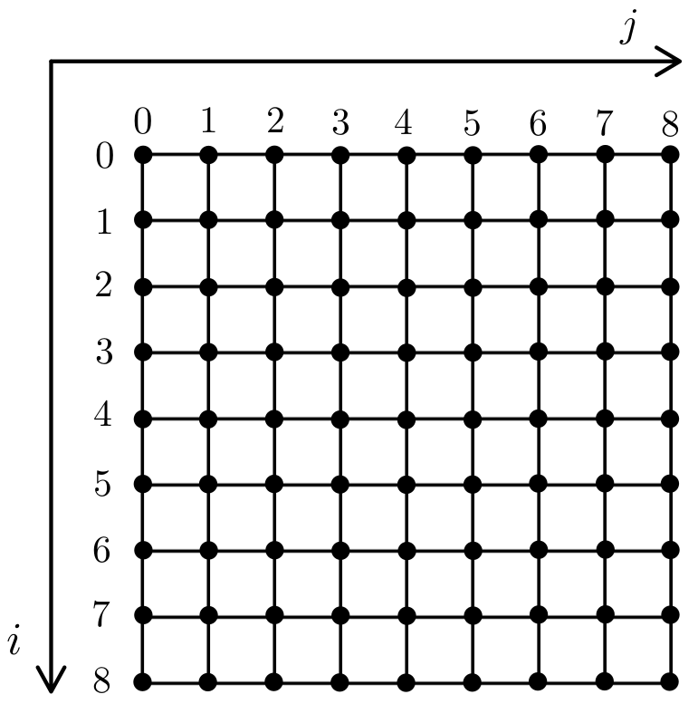
Fig.1: Points of the spatial 2D grid and its $i$ and $j$ indices as 2D Numpy array indices.

We will also consider $N_t$ time points and a time step of size $\Delta t$. Therefore, the wave function $\psi$ describing the system at a given spatial point and instant in time will be $\psi^n_{i,j}$, where $i$ and $j$ are the spatial indices that we defined previously and $n$ is the temporal index ($n=0,1,2,\dots,N_t-1$).

The Crank-Nicolson method

To obtain the essential formula of the Crank-Nicolson method we must first take a look at the “forward Euler” and “backward Euler” methods. If we consider the time derivative of a function $\psi$ as a function of $F$ discretized on the 2D plane, the derivative will be discretized by the “forward Euler” method as follows [2]:

\[\frac{\psi^{n+1}_{i,j} - \psi^n_{i,j}}{\Delta t} = F^n_{i,j}\,.\]

In the “backward Euler” method, the time derivative is discretized as [2]:

\[\frac{\psi^{n+1}_{i,j} - \psi^n_{i,j}}{\Delta t} = F^{n+1}_{i,j}\,.\]

Then, to gain stability, the Crank-Nicolson method proposes using the backward time differences and averaging with the forward time differences:

\[\frac{\psi^{n+1}_{i,j} - \psi^n_{i,j}}{\Delta t} = \frac{1}{2}\left[F^{n+1}_{i,j} + F^n_{i,j}\right] \,.\]

Discretization of the Schrödinger equation

Now we will consider the 2D time-dependent Schrödinger equation:

\[i \frac{\partial \psi(x,y,t)}{\partial t} = - \nabla^2 \psi(x,y,t) + V(x,y,t)\,\psi(x,y,t) \,.\]

For simplicity, we have considered here that $\hbar/2m = 1$, with $\hbar$ being the reduced Plank’s constant and $m$ being the mass of the considered particle. It is very important not to mistake the imaginary unit $i=\sqrt{-1}$ with the spatial index that we have seen before. Furthermore, we can also expand de $\nabla^2$ operator and write the equation as

\[i \frac{\partial \psi(x,y,t)}{\partial t} = - \left( \frac{\partial^2 \psi(x,y,t)}{\partial x^2} + \frac{\partial^2 \psi(x,y,t)}{\partial y^2} \right) + V(x,y,t)\,\psi(x,y,t)\,.\]

To discretize this equation we should remember the relationship between the indices of a 2D Numpy array and the orientation of the Cartesian axes in the Matplotlib plot. If $i$ is the row index and $j$ is the column index, we have that the relationship is

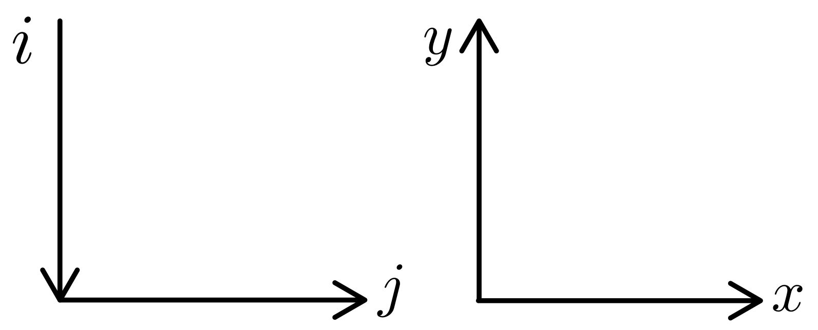
Fig.2: Relationship between the 2D Numpy array indices and the $xy$ axes orientation.

The next step is to take the finite differences version of the partial derivatives averaged in time as the Crank-Nicolson method establishes

\[\begin{array}{l} \frac{\partial \psi(x,y,t)}{\partial t} = \frac{\psi^{n+1}_{i,j} - \psi^n_{i,j}}{\Delta t}\\[2ex] \frac{\partial^2\psi(x,y,t)}{\partial x^2} = \frac{1}{2(\Delta x)^2} \left[ (\psi^{n+1}_{i,j+1} - 2\psi^{n+1}_{i,j} + \psi^{n+1}_{i,j-1}) + (\psi^{n}_{i,j+1} - 2\psi^{n}_{i,j} + \psi^{n}_{i,j-1}) \right] \\[2ex] \frac{\partial^2\psi(x,y,t)}{\partial y^2} = \frac{1}{2(\Delta y)^2} \left[ (\psi^{n+1}_{i-1,j} - 2\psi^{n+1}_{i,j} + \psi^{n+1}_{i+1,j}) + (\psi^{n}_{i-1,j} - 2\psi^{n}_{i,j} + \psi^{n}_{i+1,j}) \right]\\[2ex] V(x,y,z) \, \psi(x,y,z) = \frac{1}{2} \left[V^{n+1}_{i,j} \psi^{n+1}_{i,j} + V^{n}_{i,j} \psi^{n}_{i,j} \right] \end{array}\]

Then, we can substitute these expressions into the Schrödinger equation. We might also multiply both sides of the resulting equation by $\Delta t / i$. Then we should have the $\psi_{i,j}^{n+1} - \psi_{i,j}^n$ terms remaining on the left side of the equation. For the sake of simplicity, we now define the following constants:

\[r_x = -\frac{\Delta t}{2i(\Delta x)^2} \;, \quad r_y = -\frac{\Delta t}{2i(\Delta y)^2} \;.\]

With these two new constants, if we write the future $n+1$ wave function values in function of the present $n$ wave funtion terms we can obtain the following expression:

\[\begin{array}{l} -r_y \psi^{n+1}_{i+1,j} -r_y \psi^{n+1}_{i-1,j} + \left(1+2r_x +2r_y + \frac{i \Delta t}{2} V^{n+1}_{i,j}\right)\psi^{n+1}_{i,j} - r_x \psi^{n+1}_{i,j+1} - r_x\psi^{n+1}_{i,j-1} = \\[2ex] = r_y \psi^{n}_{i+1,j} +r_y \psi^{n}_{i-1,j} + (1 - 2r_x -2r_y - \frac{i \Delta t}{2} V^{n}_{i,j})\psi^{n}_{i,j} + r_x \psi^{n}_{i,j+1} + r_x\psi^{n}_{i,j-1} \end{array}\]

We can simplify this expression even more if we define the values

\[a_{ij} = \left(1+2r_x +2r_y + i \frac{\Delta t}{2} V_{i,j}^{n+1}\right)\]

for the left side of the equation and

\[b_{ij} = \left(1-2r_x -2r_y - i \frac{\Delta t}{2} V^{n}_{i,j}\right)\]

for the right side of the equation.

Then, we have obtained that the evolution of the wave function can be given by the formula

\[\begin{array}{l} -r_y \psi^{n+1}_{i+1,j} -r_y \psi^{n+1}_{i-1,j} + a_{i,j}\psi^{n+1}_{i,j} - r_x \psi^{n+1}_{i,j+1} - r_x\psi^{n+1}_{i,j-1} = \\[2ex] = r_y \psi^{n}_{i+1,j} +r_y \psi^{n}_{i-1,j} + b_{i,j} \psi^{n}_{i,j} + r_x \psi^{n}_{i,j+1} + r_x\psi^{n}_{i,j-1} \end{array}\]

Switching to the matrix form

This last formula can make us want to express the problem as a matrix equation of the form $\textbf{A} \cdot \textbf{x} = \textbf{b}$, where $\textbf{A}$ is a constant matrix, $\textbf{x}$ is a column vector that represents the wave function in the next time step and $\textbf{b}$ is another column vector with known independent terms. In our case, the $\textbf{b}$ column vector can be separated in two elements so that $\textbf{b} = \textbf{M} \cdot \textbf{y}$, with $\textbf{M}$ being another constant matrix and $\textbf{y}$ being a column vector representing the wave function in the present time step.

We will consider that our problem is restricted to a square 2D box (like in Fig.1) with the boundary condition of having that the wave function $\psi$ is zero at the edges of the box, that is, $\psi^n_{0,j}=\psi^n_{i,0}=\psi^n_{N-1,j}=\psi^n_{i,N-1}=0$, where $N$ was the number of points on each axis and therefore $N-1$ is the maximum value of the indices.

With this last consideration we can use the last formula of the Schrödinger equation section

to create $\textbf{A}$ and $\textbf{x}$ from the left side of the equation considering the boundary conditions:

\[\textbf{A} \cdot \textbf{x} = \begin{pmatrix} a_{00} & -r_x & 0 & 0 &\cdots & 0 & -r_y & 0 & 0 & \cdots & 0 \\[1ex] -r_x & a_{10} & -r_x & 0 &\cdots & & 0 & -r_y & 0 & \cdots & 0 \\[1ex] 0 & -r_x & a_{20} & -r_x & & & & & -r_y & \\[1ex] 0 & 0 & -r_x & \ddots & \ddots & & & & & \ddots &\\[1ex] \vdots & \vdots & & \ddots & & & & & & & \\[1ex] 0&&&&&&&&&&\\[1ex] -r_y&0&&&&&&&&&\\[1ex] 0&-r_y&&&&&&&&&\\[1ex] 0& 0&-r_y&&&&&&&\ddots&\\[1ex] \vdots& \vdots&&\ddots&&&&&\ddots&\ddots&-r_x\\[1ex] 0&0&&&&&&&&-r_x&a_{(N-1),(N-1)} \end{pmatrix} \begin{pmatrix} \psi^{n+1}_{0,0}\\[1ex] \psi^{n+1}_{1,0}\\[1ex] \psi^{n+1}_{2,0}\\[1ex] \\[1ex] \vdots \\[1ex] \\[1ex] \psi^{n+1}_{i,j}\\[1ex] \\[1ex] \vdots\\[1ex] \\[1ex] \psi^{n+1}_{(N-1),(N-1)}\\ \end{pmatrix}\,.\]

The $\textbf{A}$ matrix is composed by tridiagonal blocks of the form

\[\begin{bmatrix} a_{0,j} & -r_x & & \\[1ex] -r_x & a_{1,j} & -r_x & \\[1ex] & -r_x & a_{2,j} & \ddots & \\[1ex] & & \ddots & \ddots& -r_x \\[1ex] &&&-r_x&a_{(N-1),\,j} \end{bmatrix}\,,\]

for $j=0,1,2,…,N-1$, and diagonal blocks where there are N diagonal elements and they are equal to $-r_y$:

\[\begin{bmatrix} -r_y & & & \\[1ex] & -r_y & &\\[1ex] & &-r_y & & \\[1ex] && &\ddots& \\[1ex] &&& & -r_y \end{bmatrix}\,.\]

To check if the expressions obtained for the matrix $\textbf{A}$ and the column vector $\textbf{x}$ are correct, we can multiply $\textbf{A}$ and $\textbf{x}$ to obtain another column vector. This new column vector should have in each row expressions like the left side of our original formula.

Because the boundary conditions are set to zero at all time steps, we restrict the calculations to the indices $i,j=1,2,…,N-2$. Therefore, to leave the elements of the $\textbf{x}$ column vector as a function of one only lower index, we can define a new index

\[k = (j-1)(N-2) + (i-1)\]

so that $\psi^n_{i,j} = \psi^n_{k}$. Then, we can write $\textbf{A} \cdot \textbf{x}$ as

\[\textbf{A} \cdot \textbf{x} = \begin{pmatrix} a_{0} & -r_x & 0 & 0 &\cdots & 0 & -r_y & 0 & 0 & \cdots & 0 \\[1ex] -r_x & a_{1} & -r_x & 0 &\cdots & & 0 & -r_y & 0 & \cdots & 0 \\[1ex] 0 & -r_x & a_{2} & -r_x & & & & & -r_y & \\[1ex] 0 & 0 & -r_x & \ddots & \ddots & & & & & \ddots &\\[1ex] \vdots & \vdots & & \ddots & & & & & & & \\[1ex] 0&&&&&&&&&&\\[1ex] -r_y&0&&&&&&&&&\\[1ex] 0&-r_y&&&&&&&&&\\[1ex] 0& 0&-r_y&&&&&&&\ddots&\\[1ex] \vdots& \vdots&&\ddots&&&&&\ddots&\ddots&-r_x\\[1ex] 0&0&&&&&&&&-r_x&a_{(N-3)(N-1)} \end{pmatrix} \begin{pmatrix} \psi^{n+1}_0\\[1ex] \psi^{n+1}_1\\[1ex] \psi^{n+1}_2\\[1ex] \\[1ex] \vdots \\[1ex] \\[1ex] \psi^{n+1}_k\\[1ex] \\[1ex] \vdots\\[1ex] \\[1ex] \psi^{n+1}_{(N-3)(N-1)} \end{pmatrix}\]

Following a similar procedure, we can obtain the expression for $\textbf{M}$ and $\textbf{y}$:

\[\textbf{b} = \textbf{M} \cdot \textbf{y} = \begin{pmatrix} b_{0} & r_x & 0 & 0 &\cdots & 0 & r_y & 0 & 0 & \cdots & 0 \\[1ex] r_x & b_{1} & r_x & 0 &\cdots & & 0 & r_y & 0 & \cdots & 0 \\[1ex] 0 & r_x & b_{2} & r_x & & & & & r_y & \\[1ex] 0 & 0 & r_x & \ddots & \ddots & & & & & \ddots &\\[1ex] \vdots & \vdots & & \ddots & & & & & & & \\[1ex] 0&&&&&&&&&&\\[1ex] r_y&0&&&&&&&&&\\[1ex] 0&r_y&&&&&&&&&\\[1ex] 0& 0&r_y&&&&&&&\ddots&\\[1ex] \vdots& \vdots&&\ddots&&&&&\ddots&\ddots&r_x\\[1ex] 0&0&&&&&&&&r_x&b_{(N-3)(N-1)} \end{pmatrix} \begin{pmatrix} \psi^{n}_0\\[1ex] \psi^{n}_1\\[1ex] \psi^{n}_2\\[1ex] \\[1ex] \vdots \\[1ex] \\[1ex] \psi^{n}_k\\[1ex] \\[1ex] \vdots\\[1ex] \\[1ex] \psi^{n}_{(N-3)(N-1)} \end{pmatrix}\]

Then, having the expressions for $\textbf{A}$, $\textbf{x}$, $\textbf{M}$ and $\textbf{y}$, we can solve the equation $\textbf{A}\cdot \textbf{x} = \textbf{M}\cdot \textbf{y}\,$ for $\textbf{x}$ to obtain the wave function $\psi$ in the next time step from the wave function in the present time step (remind that $\psi^{n+1}$ is represented by $\textbf{x}$ and that $\psi^{n}$ is represented by $\textbf{y}$).

The double slit problem

To study the problem of the double slit, we first need to parametrize the slits in order to put the boundary conditions to the problem. We will use a simulation box with sides of size $L$ and infinite potential walls as we have been considering since the beginning ($\psi = 0$ at the edges).

The double slit parametrization

We define the double slit using the $i$ and $j$ indices on the grid of space points. We will also use some parameters like the width $w$ of the slit walls, the separation $s$ between slits and their aperture $a$. We can see all this more easily in the following diagram:

Fig.3: Parametrization of the double slit walls within our simulation box.

The cases that we are going to study are: the case when the double slit walls are infinite potential walls and the case when the double slit walls are finite potential barriers. We can see more details of this in the following pictures:

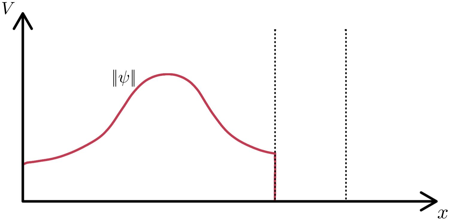
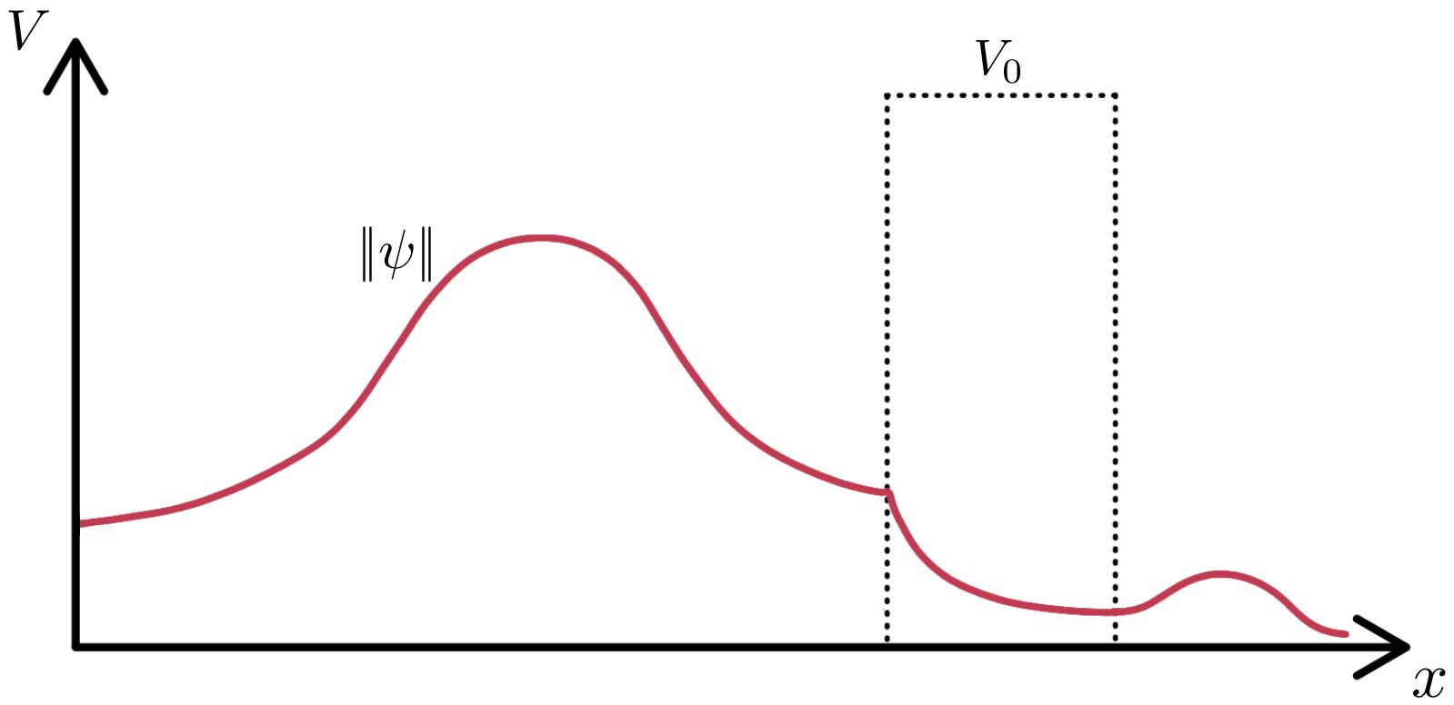
Fig.4: In the left image we can see that the wave function $\psi$ can't pass through the infinite potential wall, we have that for this case the wave function is zero inside the walls. In the image on the right we see how in this case part of the wave function manages to cross the wall of finite potential of height $V_0$.

The Gaussian wave packet

Now, the next step is to propose an initial wave function $\psi(t=0)$. For simplicity, we will consider the wave function in the initial state to be in the form of a Gaussian wavepacket. An unnormalized 1D Gaussian wavepacket centered at $x_0$ has the form

\[e^{-\frac{1}{2\sigma^2}(x-x_0)^2} \,,\]

where $\sigma$ is its standard deviation or the position uncertainty of the wavepacket.

For our 2D situation, we will consider a 2D gaussian wavepacket centered at $(x_0, y_0)$ as our initial wavefunction:

\[\psi(x,y,t=0) = e^{-\frac{1}{2\sigma^2}\left[(x-x_0)^2+(y-y_0)^2\right]} \cdot e^{-ik(x-x_0)} \,.\]

Here, we have considered that the standard deviation of the gaussian packet is the same in both $x$ and $y$ directions ($\sigma_x = \sigma_y = \sigma$). We have also introduced an additional $e^{-ik(x-x_0)}$ complex phase term with the purpose of giving initial movement to the wavepacket in the positive $x$ direction [3]. In this new term, the wavenumber $k$ is proportional to the initial momentum $p_0$ of the wavepacket, this proportionality relationship is given by the reduced Plank’s constant $\hbar$ in the form of the expression $p_0=\hbar k$ [3].

The structure of the program.

To solve the evolution of the wave function, we will need to solve the equation $\textbf{A}\cdot \textbf{x} = \textbf{M}\cdot \textbf{y}\,$ for $\textbf{x}\,$ at each time step.

In the Python script we will perform the following main steps:

Firstly, we need to define the parameters of the problem, including the indices for the parametrization of the double slit.
Then, we will fill the $\textbf{A}$ and $\textbf{M}$ matrices.
After this, we solve the evolution of the wave function. For this, we solve the equation $\textbf{A}\cdot \textbf{x} = \textbf{M}\cdot \textbf{y}\,$ for $\textbf{x}\,$ at each time step.
Lastly, we create the animation.

Results

Now the results from the calculations will be shown. In this section we can watch the resulting animations. The values of the parameters used are also indicated. It is worth remembering that the code and the animations can be found in the double-slit-2d-schrodinger GitHub repository.

The infinite potential barrier case

In this case we can see an animation of a Gaussian wavepacket passing trough a double slit with hard walls. The edges of the simulation box are hard walls too.

The parameters used for this simulation are

\[\begin{array}{l|l} L = 8 & N_t = 500\\[2ex] dx = dy = 0.05 & \sigma = 0.5\\[2ex] dt = dx^2/4 & k_x = 15 \pi \end{array}\]

The finite potential barrier case

In this other case, the following animation is the animation of a gaussian wavepacket passing trough a double slit with potential barrier walls of height $V_0=200$. The edges of the simulation box are hard walls again.

The parameters used for this simulation are

\[\begin{array}{l|l} V_0=200 & N_t = 500\\[2ex] L = 8 & \sigma = 0.5\\[2ex] dx = dy = 0.05 & k_x = 15 \pi \\[2ex] dt = dx^2/4 & \end{array}\]

For further comparison of the results with other animations, there is an animation of a double slit experiment with hard walls uploaded to Wikimedia available at [4]:

https://commons.wikimedia.org/w/index.php?title=File%3ADouble_slit_experiment.webm

References

[1] Landau, R.H., Páez Mejía, M.J. & Bordeianu, C.C., 2015. “Heat Flow via Time Stepping”. In: “Computational physics: problem solving with Python”, 3rd ed. Weinheim: Wiley-VCH.

[2] Wikipedia, 2021. “Crank–Nicolson method”. [Last time accessed January 2021] Available at: https://en.wikipedia.org/wiki/Crank%E2%80%93Nicolson_method

[3] Wheeler, N., 1998. “Gaussian Wavepackets”. Available at: https://www.reed.edu/physics/faculty/wheeler/documents/

[4] Wikipedia, 2021. “Double-slit experiment”. [Last time accessed January 2021] Available at: https://en.wikipedia.org/wiki/Double-slit_experiment

Share on

Twitter Facebook Reddit LinkedIn